
International Journal of Magnetics and Electromagnetism
(ISSN: 2631-5068)
Volume 7, Issue 1
Research Article
DOI: 10.35840/2631-5068/6533

Article Formats
Is a Propagating Infinite Plane Wave a "Radiation Field?"
Table of Content
Figures
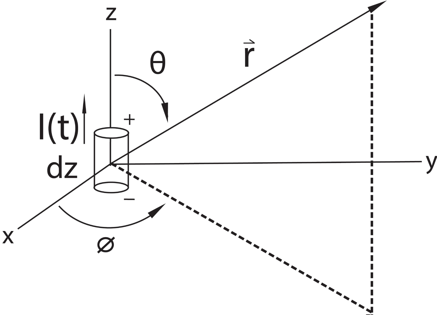
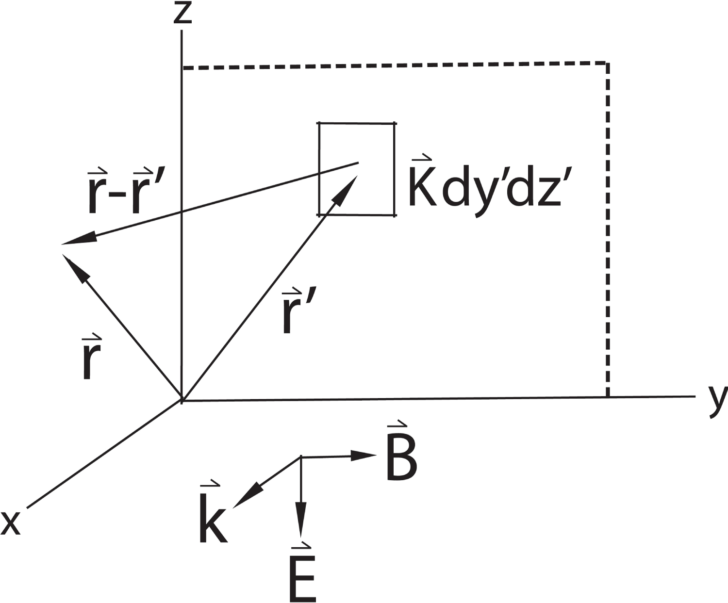
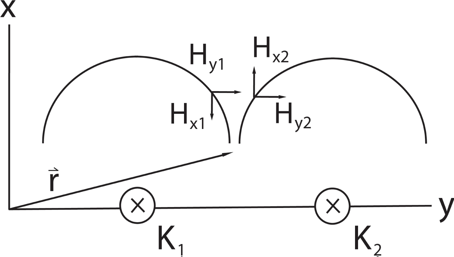
Figure 3: The Bx component from any piece of....
The Bx component from any piece of current cancels with that of an adjacent piece.
References
- Griffiths DJ (1999) Introduction to electrodynamics. (3rd edn), Prentice-Hall, Upper Saddle River, USA.
- Matthew NO Sadiku (2001) Elements of electromagnetics. (3rd edn), Oxford University Press, USA.
- Gradshteyn IS, Ryzhik IM (2007) Table of integrals, series, and products. (7th edn), Elsevier Inc, USA, 107.
- Haupt R (2003) Generating a plane wave with a linear array of line sources. IEEE Transactions on Antennas and Propagation 51: 273-278.
Author Details
W Clint Snider*, Martin A Uman and Robert C Moore
Department of Electrical and Computer Engineering, University of Florida, USA
Corresponding author
W Clint Snider, Department of Electrical and Computer Engineering, University of Florida, Gainesville, FL 32603, USA.
Accepted: May 03, 2021 | Published Online: May 05, 2021
Citation: Snider WC, Uman MA, Moore RC (2021) Is a Propagating Infinite Plane Wave a "Radiation Field?". Int J Magnetics Electromagnetism 7:033.
Copyright: © 2021 Snider WC, et al. This is an open-access article distributed under the terms of the Creative Commons Attribution License, which permits unrestricted use, distribution, and reproduction in any medium, provided the original author and source are credited.
Abstract
The total electromagnetic field of the Hertzian dipole has components that decrease with distance, r, as 1/r3, 1/r2, and 1/r. The latter component is called the "radiation field" and represents energy lost from the source. For finite-size current sources, the total distant fields can be calculated by summing just the radiation field component of the Hertzian dipoles comprising the source. We show mathematically that the propagating plane wave radiated by an infinite planar current source, composed of Hertzian dipoles, involves all field components. The nature of this paper is pedagogical: It is to clarify for electromagnetics students the semantic issues arising from discussions on radiation from antennas, in particular, radiating fields vs. radiation fields.
Introduction
The electric and magnetic fields of the Hertzian dipole, an infinitesimal time-varying current-carrying element with opposite charges residing at either end (via the continuity equation), are fundamental to the understanding of the fields of time-varying current and charge sources and, in particular, in solving for field patterns from current sources such as the half-wavelength antenna and various antenna arrays. That is, given the fields of the Hertzian dipole, one can sum (integrate) the fields of groupings of these infinitesimal current elements to determine the fields of any current source.
The standard approach to solving for the fields of the Hertzian dipole, found in most textbooks [1,2], is to recast Maxwell's Equations in the frequency domain in terms of a vector potential and a scalar potential , as
Where
Equations (1) and (2) are inhomogeneous wave equations, and eq. (3) is the Lorenz condition. is the magnetic flux density, the electric field intensity, the volume current density the volume charge density, the angular frequency, the medium permeabililty and the medium permittivity. "j" is equal to the square root of (-1).
For the case of an infinitesimal current source, the solution to in eqs. (1-5) is
for the source at the origin of a spherical coordinate system and oriented along the z-axis with length of dz, as shown in Figure 1. Application of eqs. (3-5) to (6) yields [1,2].
Hence, the fields at r are delayed a time from the time of the current, with and wave speed, c, equal to . The spherical coordinates r, θ, and φ represent, respectively, a radial distance from the origin and the zenith and azimuth angles between the origin and r. It is traditional to identify each of the terms in these equations by their radial variation from the source. The 1/r3 term is referred to as the "electrostatic field" and is present only in the electric field. It dominates the field at close distances, specifically where r is much less than the wavelength and represents the field of a time-varying point dipole. The 1/r2 dependent field, present in Bφ, Bθ, and Er, is called the "induction field" and it, along with the electrostatic terms are called the "near fields." In the case of the magnetic induction, the 1/r2 term represents the time-varying Biot-Savart law. The final terms, dependent on 1/r, are called the "radiation fields." The radiation fields are responsible for carrying energy, or radiating, away from the source and are the dominant fields where r is much greater than the wavelength. For calculating the fields of antennas on the order of wavelength size, the spatial integration of the fields of the infinitesimal dipoles, as noted earlier, need only involve the radiation fields of the source dipoles. Antenna-array field-pattern computations similarly need only consider the radiation fields. If one is far enough away from a source, or, more specifically, if the radius of curvature of the wave-front is large compared to the receiver dimension, it is a reasonable approximation to consider the spherical wave-front generated by the source to be essentially planar, although it decreases as 1/r and is not the pure or exact uniform plane wave derivable from Maxwell's Equations in Cartesian coordinates, discussed next.
The "source-free" uniform plane wave whose fields are given in eqs. (12-14) is commonly derived in Cartesian coordinates from the homogeneous Helmholtz wave equation, which is itself derived from the Maxwell curl equations with giving
Which represent a sinusoidally oscillating transverse wave with orthogonal electric, Ez(x), and magnetic, Hy(x), components traveling at the speed of light, c, in the x-direction [1,2]. No comment is made in common textbooks regarding the means by which this plane wave could be produced without a source current or, if a source current is needed, what that source current might be. Using the Hertzian dipole approach discussed above, there must be a set of infinitesimal current sources whose arrangement produces the plane wave pattern of eqs. (12-14). That this is the case may seem intuitively unreasonable, since the infinitesimal dipole source has component fields that fall off as 1/r3, 1/r2, and 1/r, the latter being called the "radiation field," whereas the "source-free" radiating plane wave of eqs. (12-14) is sinusoidally constant in amplitude with distance. Hence, the question found in this paper's title. In the next section, it is shown that multiple Hertzian dipoles can indeed be arranged to be the source of a uniform plane wave, but all dipole field components must be included in the proper calculation of the fields of the plane wave.
The Infinite Array of Hertzian Dipoles
To answer the question found in the title of this paper, we begin with the Cartesian expression for of eq. (7), written in terms of its induction and radiation components
as derived in Appendix A. The factor is the infinitesimal surface current equivalent of Idz, and it will be integrated over a large flat conductor in the yz-plane, located at as shown in Figure 2. As follows from eq. (15-16) and Figure 3, any -field component in the direction is canceled by a directed component from a little piece of current equidistant in the opposite direction from the field point. It follows that the field components may then be written as
Where the origin may be placed anywhere on the infinite sheet, so we let y = z = 0. A cylindrical substitution, is then made to facilitate the integration. The new limits on the integral(s) are and . The factor in both terms will be defined as . Thus
If we let , and replace the limits, the integrals become
Which can be found in integral tables [3]. The above integrals yield
Where,
is the exponential integral [3]. In summing eq. (25) and eq. (26), the two exponential integral terms from each equation cancel one another, and as , the first term in eq. (25) goes to zero, leaving only the third term in . When we replace by its definition
and using Maxwell's equation gives
Which is equivalent to eqs. (12-13) with
being the amplitudes of the wave components in eqs. (12-13) and η keeping its definition from eq. (14). It is clear from the summation of eqs. (25) and (26), that both the radiation and the induction fields of the dipoles are involved in producing the uniform plane wave (whose amplitude does not decay with distance). Thus, the radiating plane wave is not a radiation field.
Discussion and Conclusion
According to the calculations of section II, the radiation field components of the dipoles comprising the plane wave source do not solely make up the fields that propagate; Parts of the magnetic induction field cancel parts of the magnetic radiation field. Presumably, the electric field of the radiating plane wave is composed of all three dipole fields components.
The fact that all dipole field components are involved in the plane wave is a consequence of the infinite size of the source. To be in the far-field of all of the dipoles together would require being an infinite distance from the source.
Although a current source of infinite extent is not practical, some reasonable approximate plane-wave-generating devices have been constructed from multiple dipoles [4]. The primary technical requirement is in the phasing of each dipole which makes up the sheet. Each dipole needs to have an identical current, in both magnitude and phase.
An alternate and simpler, but less pedagogically satisfying derivation of the plane wave from the infinite current sheet, using directly, is given in Appendix B.
Finally, the calculation of the fields of an infinite current source, as given in the body of this paper and in Appendix B, is not commonly found in textbooks and probably should be, given that it illuminates the nature of the seemingly understood definitions of radiation and radiating.